
With AKTU’s Question Paper, you may embark on an Exciting Geotechnical Engineering Journey. Improve your understanding, test your knowledge, and fly to exam achievement.
Dudes 🤔.. You want more useful details regarding this subject. Please keep in mind this as well.

Important Questions For Geotechnical Engineering:
*Quantum          *B.tech-Syllabus
*Circulars           *B.tech AKTU RESULT
* Btech 3rd Year
Section A: Short Question In Geotechnical Engineering
a. Explain the flow curve.
Ans. The water content is used as the ordinate and the number of blows on the log scale as the abscissa in a plot. Flow curve is the name of this diagram. This is used to determine a soil’s liquid limit.
b. Differentiate cohesive and cohesionless soil.
Ans.
| S. No. | Cohesive Soil | Cohesionless Soil |
| 1. | Cohesive soils are those in which the interaction of adsorbed water and particle attraction causes plastic deformation at different water contents. | The soils composed of bulky grains are cohesionless. |
| 2. | Example: Clays, plastic silt. | Example: Non plastic silt, coarse grained soils. |
c. Write flow equation for anisotropic soil.
Ans. Flow equation for anisotropic soil,
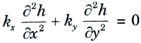
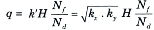
Hence the discharge is given by,
d. Write assumptions for Laplace equation.
Ans. Assumptions made for Deriving the Laplace Equation:
- 1. The flow is two dimensional.
- 2. Water and soil are incompressible.
- 3. Soil is isotropic and homogeneous.
- 4. The soil is fully saturated.
- 5. The flow is steady, i.e., flow conditions do not change with time.
- 6. Darcy’s law is valid.
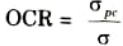
e. Define over-consolidation ratio.
Ans. Over consolidation ratio is defined as the ratio of the preconsolidation stress (𝜎pc) to the current effective stress (𝜎).
f. Discuss the secondary consolidation.
Ans.
- 1. Even after the surplus hydrostatic pressure created by the applied pressure has completely dissipated and the primary consolidation is finished, the volume decrease still happens at a very sluggish rate.
- 2. The next volume reduction is referred to as secondary consolidation.
- 3. It is ascribed to the solid particles’ plastic readjustment and the water’s absorbed water to the new stress system.
g. Write the assumptions of Westergaard theory.
Ans. Following are the assumptions of Westergaard’s theory:
- i. The soil is elastic and semi-infinite.
- ii. Soil is composed of numerous closely spaced horizontal layers of negligible thickness of an infinite rigid material.
- iii. The rigid material permits only the downward deformation of mass in which horizontal deformation is zero.
h. Write the limitations of triaxial test.
Ans. 1. The apparatus is elaborate, costly and bulky.
2. In comparison to a direct shear test, the drained test requires more time.
3. The assumption that the specimen will remain cylindrical does not hold up well at enormous strains, making it impossible to precisely calculate the cross-sectional area of the specimen.
i. Discuss the rotational failure of slope.
Ans. i. As depicted in Fig., this form of failure rotates over a slip surface as the soil mass moves outward and downward.
ii. In cases of homogenous soil conditions, the slip surface is typically circular, while in cases of non-homogeneous soil conditions, it is non-circular.
j. Write the assumptions of Rakine’s earth pressure theory.
Ans. Assumptions: Following are the assumptions made by Rankine for the derivation of earth pressure:
- 1. The soil mass is homogeneous and semi-infinite.
- 2. The soil is dry and cohesionless.
- 3. The ground surface is plane, which may be horizontal or inclined.
- 4. The back of the retaining wall is smooth and vertical.
- 5. The soil element is in a state of plastic equilibrium, i.e., at the verge of failure.
Section B :
a. Illustrate the various structures of Soil.
Ans. Soil Structure:
- 1. The organization and state of aggregation of soil particles in a soil mass is the typical definition of soil structure.
- 2. This term encompasses, in a broader sense, consideration of the ionic composition, nature, and properties of soil water as well as the forces at play between soil particles, soil water, and their adsorption complexes. It also refers to the shape and orientation of solid particles as well as their electrical and mineralogical composition.
- 3. In terms of structure, soil particles include both the aggregates or structural elements that are created by the accumulation of smaller mechanical fractions, such as sand, silt, and clay, as well as the individual mechanical components, such as sand, silt, and clay.
- 4. Soil structure is an important factor which influences many soil properties, such as permeability, compressibility and shear strength etc.
- 5. Following are the various types of soil structure:
- i. Single Grained: An arrangement composed of individual soil particles.
- ii. Honeycomb:
- a. A configuration of soil particles that resembles a honeycomb and is rather free and stable.
- b. Regardless of how the particles are distributed within the bundles, the soil mass is made up of loosely arranged bundles of particles.
- iii. Flocculent: A configuration made up of soil particle flocs rather than single soil particles. Edge-to-edge or edge-to-face with respect to one another is how the particles are positioned.
- iv. Dispersed: An arrangement composed of particles having a face-to-face’ or parallel orientation.
- v. Coarse Grained Skeleton: A configuration of coarse grains acting as a skeleton, with a rather loose assemblage of the finest soil grains filling the spaces.
- vi. Cohesive Matrix: A configuration that prevents coarse fraction particle-to-particle interaction. Within a substantial mass of cohesive fine grains, the coarse grains are still there.
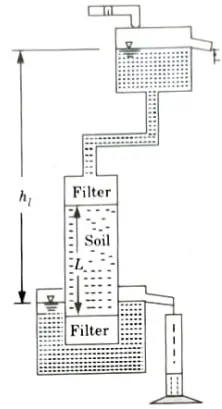
b. Demonstrate the constant head permeability test.
Ans.
- i. Constant-head tests are used for estimating the coefficient of permeability of coarse-grained soils of high permeability, such as clean Sands and gravel.
- ii. Fig. shows the arrangement in which the flow is one-dimensional and in downward direction.
- iii. The figure also indicates the head loss (hl) and the corresponding length of soil, L, over which the head loss occurs.
- iv. The experimental data consist of a measured quantitý of discharge Q during a time interval t, under steady state conditions of flow. The head loss hl is also noted.
- v. k can be computed from the formula,
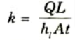
where, Q = Quantity of discharge in time t.
hl = Head loss over length L.
A = Area of cross-section of soil sample.
Limitations: Following are the limitations of constant head permeability test:
- i. Equipment expensive.
- ii. Complicated to set up and to use.
- iii. Not suitable for most sites.
- iv. Test duration long.
c. Explain the Terzaghi’s theory of consolidation.
Ans. Following are the assumptions made in Terzaghi’s one dimensional consolidation theory:
- 1. The mass of soil is uniform and completely soaked.
- 2. Water and dirt granules are incompressible.
- 3. During consolidation, Darcy’s law, which governs how water moves through soil masses, is applicable.
- 4. During consolidation, the coefficient of permeability remains constant.
- 5. Just one direction of load application is made, and only that direction experiences deformation.
- 6. The volume reduction is the only cause of the deformation.
- 7. Pore water can only be discharged in one direction.
- 8. The flow of water from the soil encounters no resistance at a boundary drainage face.
- 9. Although there is continual thickness change during consolidation, the final amount of compression is simply related to the initial thickness.
d. Illustrate Culmann’s construction for active pressure.
Ans. Culmann’s Graphical Method:
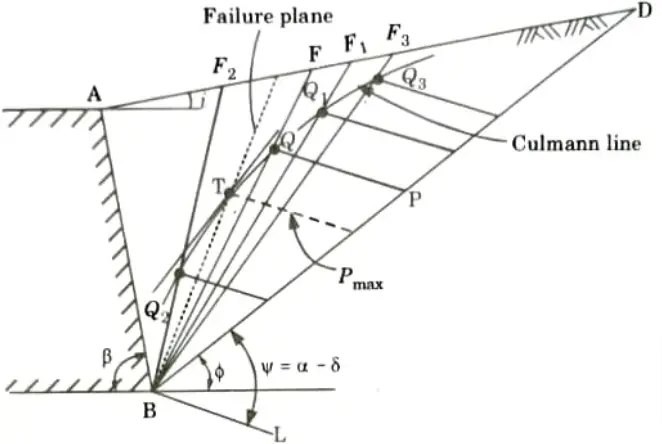
- 1. Rehbann’s construction becomes inconvenient when the slope angle i approaches the angle 𝛟’. Culmann developed a method which is more general than Rehbann’s method.
- 2. For soils lacking cohesiveness, Culmann’s approach is practical for calculating the active earth pressure. In actuality, the majority of backfills fall within this group.
- 3. The technique is applicable to backfill surfaces with any form, various surcharge weights, and even stacked backfill.
The Procedure Consists of the Following Steps:
- 1. Draw the retaining wall AB to the scale.
- 2. Draw the 𝛟-line BD.
- 3. A line BL is drawn at an angle 𝛹 with line BD, such that 𝛹 = 𝛼 – 𝛿.
- 4. A failure surface BP is assumed, and the weight (W) of failure wedge ABF is computed.
- 5. The weight (W) is plotted along BD such that BP = W
- 6. A line PQ is drawn from point parallel to BL to intersect the surface BF at Q.
- 7. The length PQ represents the magnitude of Pa required to maintain equilibrium for assumed failure plane.
- 8. Several other failure planes BP2, BR1, BR3, etc., are assumed and the procedure is repeated. Thus, the point Q2, Q1, Q3, etc., are obtained.
- 9. A smooth curve is drawn joining points Q2, Q, Q1, Q3 etc. The curve is called Culmann’s line.
- 10. A line (shown dotted) is drawn tangential to the Culmann line and parallel to BD. Point T is the point of tangency.
- 11. The magnitude of the largest value (Pmax) of Pa is measured from the tangent point ‘T’ to the line BD and parallel to BL. It is equal to Coulomb’s pressure (Pa).
- 12. The actual failure plane passes through the point T (shown dotted).
e. Discuss the Taylor’s stability number.
Ans.
- 1. This dimensionless number is proportional to the required cohesion and is inversely proportional to the allowable height.
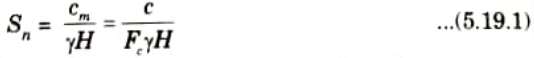
- 2. The reciprocal of the stability number is known as stability factor.
- 3. Taylor determined the values of Sn for finite slopes using the friction circle method.
- 4. The charts are prepared indicating the stability number, and slope angle i for various values of 𝛟m as shown in Fig.
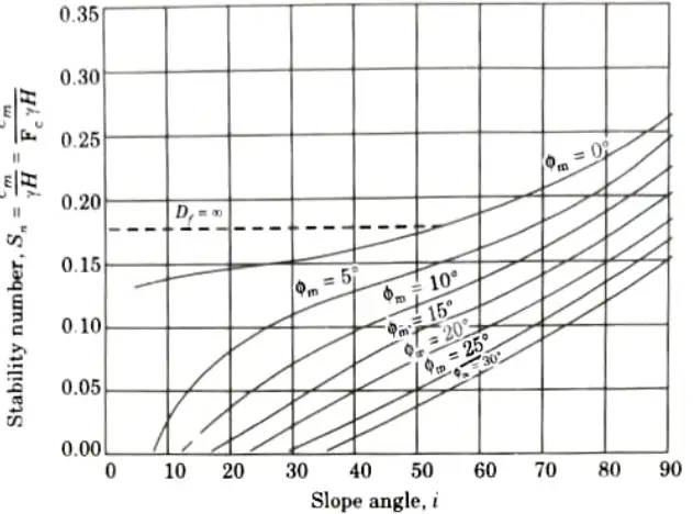
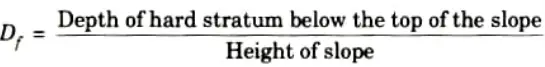
- 5. There are 5 parameters, viz cm, 𝛶, H, i and 𝛟m. However, if 𝛟m =0 (purely cohesive soils), a sixth parameter Df becomes also important, as shown in Fig.
Section 3 : Long Question
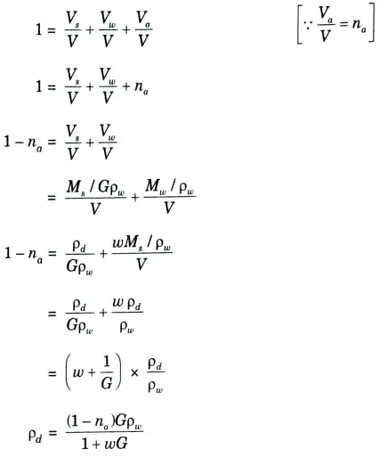
a. Derive the relation:
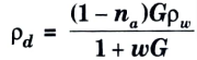
Ans. 1. Volume of soil,
V = Vs + Vw + Va
2. Divided by V,
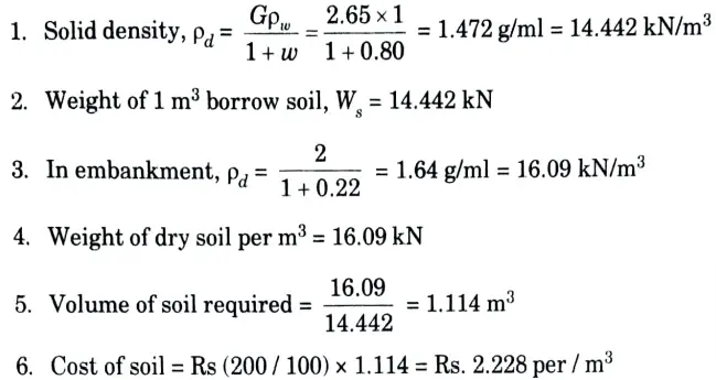
b. There are two borrow areas A and B which have soils with void ratios of 0.80 and 0.70, respectively. The in-place water content is 20 %, and 15 %, respectively. The fill at the end of construction will have a total volume of 10,000 m3, bulk density of 2 Mg/m3 and a placement water content of 22 % Determine the volume of the soil required to be excavated from both areas. G = 2.65.
If the cost of excavation of soil and transportation is Rs. 200/- per 100 m3 for area A and Rs. 220/- per 100 m3 for area B, which of the borrow area is more economical?
Ans. Given: Void ratio, eA = 0.80, eB = 0.70, Water content, wA = 20%, wa = 15%, Total volume, V = 10000 m3, Bulk density, 𝜌 = 2 Mg/m3, After fill, water content, w = 22%, Specific gravity, G = 2.65, Cost of excavation of soil transportation for A = 200 Rs/ 100 m3, For B = 220 Rs/100 m3
To Find: Volume of the soil required to be excavated.
A. For Borrow Area A:
B. For Borrow Area B:

2. Ws = dry weight/m3 = 15.304 kN
3. In embankment, weight of dry soil = 16.09 kN
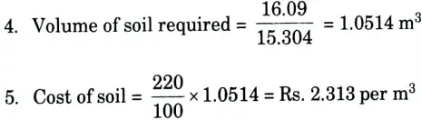
C. Borrow area A is more economical.
Section 4 : Important Question
a. In a constant head permeameter test, the following observations were taken.
Distance between piezometer toppings =100 mm
Difference of water levels in piezometers = 60 mm
Diameter of the test sample = 100 mm
Quantity of water collected = 350 ml
Duration of the test = 270 seconds
Determine the coefficient of permeability of the soil.
Ans. Given: Distance between piezometer toppings = 100 mm, Difference of water levels in piezometer = 60 mm, Diameter of the test sample, d = 100 mm, Quantity of water collected = 350 ml, Duration of the test = 270 sec.
To Find: Determine the coefficient of permeability of the soil.
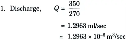
2. Coefficient of permeability,
k = QL/Ah
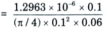
= 2.75 x 10⁻⁴ m/sec
= 0.0275 cm/sec
b. Explain the process for construction of flow net for determination of discharge through a dam. Discuss the applications of flow net briefly.
Ans. A. Process: The procedure for drawing the flow net can be divided into the following steps:
- 1. First identify the hydraulic boundary conditions. In Fig. 2, the upstream bed level GDAK represents 100 % potential line and the downstream bed level CFJ, 0% potential line. The first flow line KLM hugs the hydraulic structure and is formed by the flow of water on the upstream of the sheet pile and at the interface of the base of the dam and the soil surface. The last flow line is indicated by the impervious stratum NP.
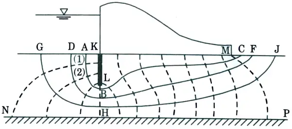
- 2. Next to the boundary line, draw a test flow line ABC. The line must be perpendicular to the beds in the upstream and downstream directions.
- 3. Beginning at the upstream end, draw equipotential lines to roughly divide the first flow channel into squares. The square should progressively increase in size.
- 4. Extend the equipotential lines that make up the squares’ sides downward. These extensions identify the squares’ approximate widths, such as the squares with the numbers (1) and (2). The widths as decided above are set as the other square sides. The following flow line DF is then created connecting these bases after irregularities have been smoothed down. It is important to take care when sketching the flow line to make the flow fields roughly square throughout.
- 5. The equipotential lines are further extended downward, and one more flow line GHJ is drawn, repeating the step, (4).
- 6. If the flow fields in the last flow channel are inconsistent with the actual boundary conditions, the whole procedure is repeated after taking a new trial flow line.
B. Application: Flownet is used to:
- 1. Estimation of seepage losses from reservoir.
- 2. Determination of seepage pressure.
- 3. Uplift pressure below dams.
- 4. To check against the possibility of piping and many others.
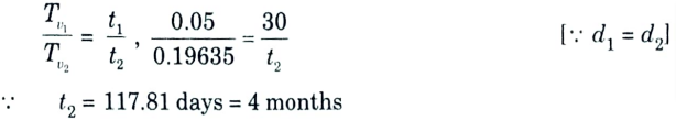
a. A clay layer whose total settlement under a given loading is expected to be 12 cm settles 3 cm at end of 1 month after application of load increment. How many months will be required to reach settle of 6 cm. Assume layer to have double drainage.
Ans. Given: Total settlement 12 em, 30 days after settlement 3 cm Double drainage.
To Find: Time required to settlement of 6 cm.
1. Percentage settlement after 1 month,
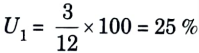
2. Time factor for U< 60% is given by,
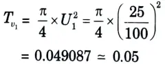
3. Percentage settlement,
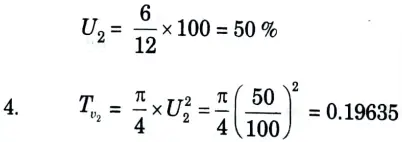
5. Time factor is also given by,

7. From eq. (i) and eq. (ii), we get
b. Explain the process involved in determination of compaction in light and heavy compaction test.
Ans. A. Process of Light Compaction Test:
- 1. Take a representative sample weighing approximately 20 kg of thoroughly mixed air dried material passing 4.75 mm (or 20 mm) IS sieve. Add enough water to bring its water content to about 7 percent (sandy soils) or 10 percent (clayey soils) less than the estimated optimum moisture content. Keep this soil in an air tight container for about 20 hours, for maturing.
- 2. Clean the mould and fix it to the base. Take the empty mass of the mould and the base, nearest to 1g.
- 3. Attach the collar to the mould. The inside of the mould may be greased thoroughly.
- 4. Procedure:
- i. Mix the matured soil thoroughly. Take out about 2(1/2)kg of the soil and compact it in the mould in three equal layers, each layer being given 25 blows from the rammer weighing 2.6 kg dropping from a height of 310 mm, if 1000 ml. mould is used.
- ii. If however, the 2250 ml mould is used, about 5 kg of soil should be taken and should be compacted in three equal layers, each layer being given 56 blows from the rammer weighing 2.6 kg dropping from a height of 310 mm.
- iii. Each layer’s surface should receive blows that are evenly spaced across it. Prior to adding the soil for the subsequent layer, each layer of compacted soil should be scored with a spatula.
- iv. The soil should only be used to fill the mould, leaving around 5 mm to be removed when the collar is taken off.
- v. Use the Proctor’s needle to determine the penetration resistance of compacted soil.
- vi. Take off the collar and use a straight edge to trim the extra soil. The mould should be cleaned from the exterior and weighed to the nearest gramme. Remove the soil from the mould, slice it in half, and save a representative soil sample for measuring its water content.
- 5. Repeat steps 4 for about five or six times, using a fresh part of the soil specimen and after adding higher water content than the preceding specimen.
- 6. The dry density of the compacted soil is calculated as follows:
B. Heavy Compaction (Modified Proctor’s Test) Test:
- 1. The heavy compaction test requires the same equipment as the light compaction test, with the exception that the rammer has a falling mass of 4.9 kg and a drop of 45 cm.
- 2. Instead of three equal layers, the dirt is compressed into five. If a 1000 ml mould is used, each layer receives 25 rammer blows, and if a 2250 ml mould is used, each layer receives 55 rammer blows.
3. Procedure: Same as light compaction test.
Section 6 : Important Question
a. A given saturated clay is known to have effective strength parameters of C’ = 10 kPa and 𝜑’ = 28°. A sample of this clay was brought to failure quickly so that no dissipation of the pore water could occur at failure it was known that

i. Estimate the values of 𝜎1 and 𝜎3 at failure.
ii. What was the effective normal stress on the failure plane?
Ans. Given: Effective strength parameter, C = 10 kPa, 𝛟’ = 28°, 𝜎1’ = 60 kPa, 𝜎3’ = 10 kPa and uf = 20 kPa
To Find: Value of 𝜎1 and 𝜎3 at failure and effective normal stress at failure plane.
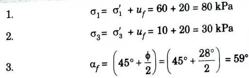
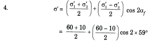
= 23.263 kPa
b. A long strip footing of width 2 m carries a load of 400 kN/m. Calculate the maximum stress at a depth of 5 m below the centre line of the footing. Compare the results with 2:1 distribution method.
Ans. Given: Width of strip, w = 2m, Load, l = 400 kN/m, Depth, 2 = 5m
To Find: Calculate the maximum stress, compare the result with 2:1 distribution method.
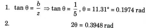
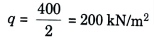
3. Intensity of load per m2,
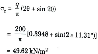
4. Stress at depth z is given by,
5. 2:1 distribution method.
Stress is given by,
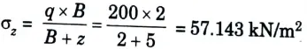
6. 2:1 distribution method produce more value of stress.
Section 7 : Important Question
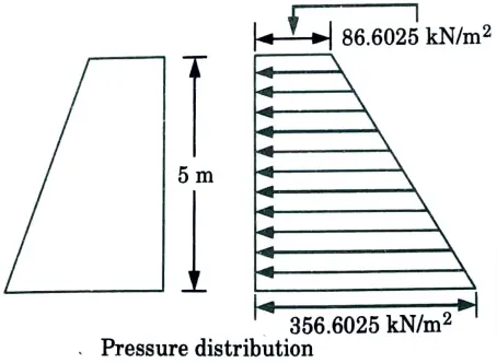
a. A smooth vertical 5 m high retains a soil with c = 2.5 N/cm2, 𝜑 = 30, and 𝛶 = 18 kN/m3. Show the Rankine passive pressure distribution and determine the magnitude and point of application of the passive resistance.
Ans. Given: Height of wall, h =5m, Cohesion, c = 2.5 N/cm2, Bulk unit weight, 𝛶 = 18 kN/m3, 𝛟 = 30°
To Find: Rankine pressure distribution, Value of passive pressure and point of application.
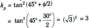
1. Coefficient of passive pressure,
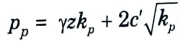
2. Passive pressure is given by,
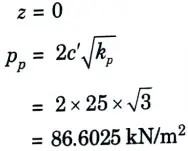
3. At depth,
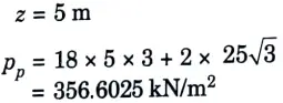
4. At depth,
5. The total pressure on the retaining wall of height H is given by,
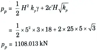
6. Point of application,
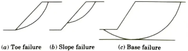
b. Discuss the stability of slope. Explain various types of slope failure with neat sketches.
Ans. A. Stability of Slope:
1. Determining how much force a specific slope can withstand before failing is the process of slope stability.
2. Commercially used highways, dams, excavated slopes, and soft rock routes in reservoirs, forests, and parks are a few examples of common slopes.
3. A slope is seen as stable if it can withstand movement, whereas it is regarded as unstable if the movement is too great for the slope.
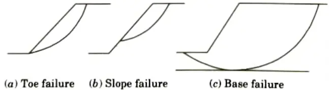
B. Types of Slope Failure: Following are the various types of slope failures:
1. Rotational Failure:
i. As depicted in Fig., this form of failure rotates over a slip surface as the soil mass moves outward and downward.
ii. In cases of homogenous soil conditions, the slip surface is typically circular, while in cases of non-homogeneous soil conditions, it is non-circular.
2. Translational Failure:
i. A constant slope of unlimited extent and having uniform soil properties at the same depth below the free surface is known as an infinite slope.

ii. Translational failure occurs in an infinite slope along a long failure surface parallel to the slope, as shown in Fig.
3. Compound Failure:
i. A compound failure is a combination of the rotational slips and the translational slip, as shown in Fig.
ii. A compound failure surface is curved at the two ends and plane in the middle portion.

4. Wedge Failure: As depicted in Fig., a failure along an inclined plane is referred to as a block, wedge, or plane failure. It happens when discrete soil mass wedges and blocks separate from one another.
5. Miscellaneous Failures: In addition to the aforementioned four failure types, complicated failure types in the form of spreads and flows may also take place.
6 thoughts on “Geotechnical Engineering: Last year Question Paper Questions with Answer”