
A Machine Learning Technique, like a clever robot friend, is a smart computer program that learns from data to help with problem-solving and decision-making. AKTU Solved Question Paper provides comprehensive test preparation tools. Join us on this educational adventure!
Dudes 🤔.. You want more useful details regarding this subject. Please keep in mind this as well.

Important Questions For Machine Learning Techniques:
*Quantum          *B.tech-Syllabus
*Circulars           *B.tech AKTU RESULT
* Btech 3rd Year
Section A: Aktu Short Questions with Answers
a. What is a “Well -posed Learning” problem ? Explain with an example.
Ans. A well-posed learning issue is one that has a unique solution, depends on data, and is not sensitive to minute data changes.
The three important components of a well-posed learning problem are Task, Performance Measure and Experience.
For examples, Learning to play Checkers:
A computer might enhance its capabilities so that it can succeed at the category of activities that involve playing checkers. By practise and competition with itself, the performance keeps getting better.
To simplify,
T->Play the checkers game.
P-> Percentage of games won against the opponent.
E-> Playing practice games against itself.
b. What is Occam’s razor in ML ?
Ans. According to Ocam’s razor, we should choose simpler models with fewer coefficients over complicated models when using machine learning. A heuristic states that more complicated hypotheses tend to include more assumptions, which will make them excessively specific and hinder their ability to generalize.
c. What is the role of Inductive Bias in ANN?
Ans. An significant factor in the ability of ANN to generalize to previously unknown data is inductive biases. The set of presumptions the learner employs to forecast outputs of given inputs that it has not yet experienced is known as the inductive bias (also known as learning bias) of a learning algorithm.
d. What is gradient descent delta rule ?
Ans. Gradient descent: Gradient descent is an optimisation technique that iteratively moves in the direction of the steepest descent, as indicated by the gradient’s negative, in order to minimize some function.
Delta rule: Gradient descent is simply applied using the delta rule. If the training examples are not linearly separable, it converges towards a best-fit approximation to the target notion.
e. What is Paired t-Tests in Hypothesis evaluation ?
Ans. Gradient descent is simply applied using the delta rule. If the training examples are not linearly separable, it converges towards a best-fit approximation to the target notion.
f. How do you find the confidence interval for a hypothesis test?
Ans. Data from a sample is used to estimate a population parameter using confidence intervals. Data from a sample is used in hypothesis testing to examine a given hypothesis. The hypothesis tests work hand in hand with confidence intervals. Typically, the conclusion reached using the confidence interval is the same as the one reached using the hypothesis test. In other words, a hypothesis test at the 0.05 level will virtually always fail to reject the null hypothesis if the 95% confidence interval contains the hypothesised value. A hypothesis test at the 0.05 level will nearly certainly reject the null hypothesis if the 95% confidence interval does not include the hypothesised parameter.
g. What is sample complexity of a Learning Problem ?
Ans. The number of training samples we must give the method to ensure that the function it returns is within an arbitrarily tiny error of the best feasible function, with probability arbitrarily near to 1, is known as sample complexity.
h. Differentiate between Lazy and Eager Learning.
Ans.
| S. No. | Lazy learning | Eager learning |
| 1. | Lazy learning techniques merely store the data, delaying generalisation beyond these facts until a specific request is made. | Based on the given training examples, eager learning approaches create a general, explicit description of the goal function. |
i. What is the problem of crowding in GA?
Ans.
- 1. In genetic algorithms, crowding preserves population variety by mating each progeny with a comparable person already existing in the population (pairing phase), and then determining which of the two will survive (replacement phase).
- 2. Deterministic or probabilistic crowding is typically used for the replacement phase of crowding, although both have the drawback of exerting the same selective pressure regardless of the nature of the problem being solved or the stage of genetic algorithm search.
j. Comparison of purely analytical and purely inductive learning.
Ans.
| S. No. | Purely analytical learning | Purely inductive learning |
| 1. | Information for inductive learning is gathered through observation. | Analytical learning information is obtained by explaining and analyzing these observations. |
| 2. | In order to learn in situations when prior knowledge is partial or inaccurate, inductive learning mechanisms are required. | Analytical learning methods are necessary to scale up to understanding complicated ideas and to deal with circumstances where available training data is restricted. |
Section B: Long Questions With Solutions
a. Design the Final design of checkers learning program.
Ans. A. Steps for designing checkers learning program are:
- 1. Choosing the Training Experience
- 2. Choosing the Target Function
- 3. Choosing a Representation for the Target Function
- 4. Choosing a Function Approximation Algorithm
- 5. The Final Design
B. Design of the final design of checkers learning program:
- 1. The performance System:
- i. Using the learnt target function, solve the provided performance problem (s).
- ii. It accepts a new board as input and returns a trace of the game it played against itself.
- 2. The Critic:
- i. To take the game’s history or trace as input and provide a series of training instances of the target function as output.
- 3. The Generalizer:
- i. Using the training examples as input, generate an output hypothesis that is an estimate of the target function.
- ii. It generalizes from specific training examples, hypothesising a general function that includes examples as well as cases other than the training examples.
- iii. Effective generalization to new cases is critical.
- 4. The Experiment Generator:
- i. Takes the current hypothesis (currently learnt function) as input and generates a fresh challenge for the performance system to explore (an initial board state).
- ii. Its duty is to select fresh practise problems that will maximise the overall system’s learning rate.
b. What is Maximum Likelihood and Least Squared Error Hypothesis ?
Ans. A. Maximum Likelihood Hypothesis:
1. A typical modelling difficulty is determining how to estimate a dataset’s joint probability distribution.
2. This challenge is made more difficult by the fact that the sample (X) selected from the population is tiny and noisy.
3. Maximum Likelihood Estimation is one approach to probability density estimation.
4. Maximum Likelihood Estimation entails approaching the problem as an optimisation or search problem, in which we seek a set of parameters that results in the greatest fit for the data sample’s joint probability (X).
5. First, it entails defining a parameter called theta, which specifies both the probability density function and the distribution’s parameters. It is formalized as:
P (X ; theta)
6. This conditional probability is known as the likelihood of witnessing the data given the model parameters and is denoted by the notation L() to signify the likelihood function. As an example:
L(X ; theta) (X ; theta)
7. The goal of Maximum Likelihood Estimation is to identify the set of parameters (theta) that maximise the likelihood function, i.e., produce the highest likelihood value.
L should be maximized
(X ; theta)
B. Least Squared Error Hypothesis:
- 1. The least-squares method is a common technique in regression analysis.
- 2. It is a mathematical method for determining the best fit line for a relationship between an independent and dependent variable.
- 3. Several learning methods, including neural network learning, linear regression, and others, attempt to learn a continuous-valued goal function.
- 4. If certain conditions are met, any learning technique that minimizes the squared error between the output hypothesis predictions and the training data will produce a Maximum Likelihood Hypothesis.
- 5. This conclusion is significant because it gives a Bayesian basis (under certain assumptions) for curve fitting approaches that aim to minimize the sum of squared errors over the training data.
c. What problem does the EM algorithm solve ?
Ans. Following are the problem that EM algorithm solve:
- 1. When some data is missing, the EM technique is employed to derive maximum likelihood estimates of parameters.
- 2. The EM technique can also be used when there is latent data, i.e. data that was never meant to be noticed in the first place.
- 3. The EM technique is used in Bayesian statistics to determine the mode of the posterior marginal distributions of parameters.
d. Highlight the importance of Case Based Learning.
Ans.
- 1. Ease of knowledge elicitation
- 2. Absence of problem-solving bias
- 3. Incremental learning
- 4. Suitability for complex and not-fully formalized solution spaces
- 5. Suitability for sequential problem solving
- 6. Ease of explanation
- 7. Ease of maintenance
e. Write short notes on Learning First Order Rules.
Ans.
- 1. Individual propositions and their truth-functional combinations can be expressed using propositional logic.
- 2. First order logic allows us to state propositions and their truth functional combinations, but it also allows us to express propositions as assertions of predicates about individuals or groups of individuals.
- 3. Inference rules allow for the drawing of inferences about sets/individuals.
- 4. First order logic is far more expressive than propositional logic, allowing for finer-grained definition and reasoning when representing knowledge.
- 5. Learners of first order rules can generalize to relational ideas (which propositional learners cannot).
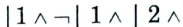
- 6. All expressions in first-order logic are composed of the following attributes:
- i. Constants – e.g. Tyler, 23, a
- ii. Variables – e.g. A, B, C
- iii. Predicate symbols – e.g. male, father (True or False values only)
- iv. Function symbols – e.g. age (can take on any constant as a value)
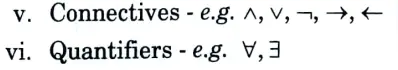
- vii. Term: It can be defined as any constant, variable or function applied to any term. E.g. age(bob).
- viii. Literal: It can be defined as any predicate or negated predicate applied to any terms, e.g, female(sue), father(X, Y).
Section 3: “Concept Learning”
a. Explain the “Concept Learning” task giving an example.
Ans.
- 1. The idea Finding the hypothesis that best fits the training examples can be thought of as a task of searching through a predefined space of potential hypotheses.
- 2. The search can be effectively organized by utilizing a naturally occurring structure over the hypothesis space, which contains a general-to-specific ordering of hypotheses.
- 3. Concept Learning can be understood from following example:
A concept learning task – Enjoy sport training example:
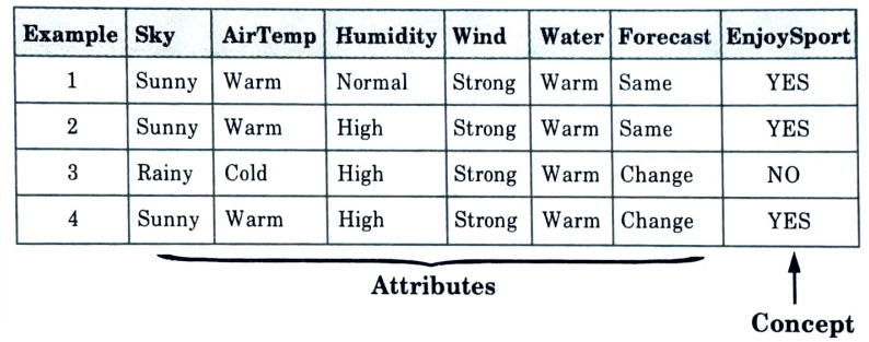
- 4. A list of example days, each of which is defined by six characteristics.
- 5. Based on the values of its attribute values, the aim is to learn to anticipate the value of EnjoySport for every given day.
- 6. A confluence of restrictions on the instance attributes makes up each hypothesis.
- 7. Each hypothesis will be a vector of six constraints, specifying the values of the six attributes – (Sky, AirTemp, Humidity, Wind, Water, and Forecast).
- 8. Each attribute will be:
? – indicating any value is acceptable for the attribute (don’t care) single value – specifying a single required value (e.g. Warm) (specific)
0 – indicating no value is acceptable for the attribute (no value)
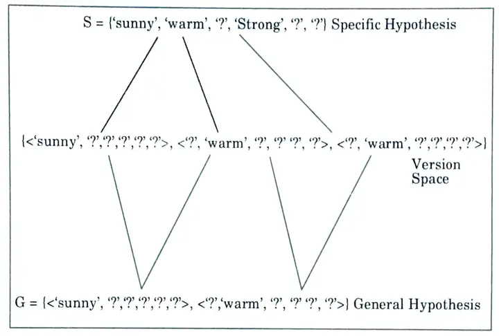
b. Find the maximally general hypothesis and maximally specific hypothesis for the training examples given in the table using the candidate elimination algorithm.
Given Training Example:
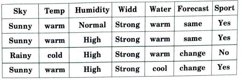
Ans. Step 1:
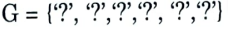
Initialize G & S as most General and specific hypothesis.
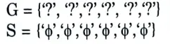
Step 2:
for each +ve example make a specific hypothesis more general.
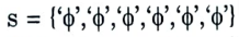
Take the most specific hypothesis as your 1st positive instance.
h = {‘sunny’, ‘warm’, ‘Normal’, ‘Strong’, ‘warm’, ‘same’}
General hypothesis will remain same :
Step 3:
Compare with another positive instance for each attribute.
if (attribute value = hypothesis value) do nothing.
else
replace the hypothesis value with more general constraint ‘?’.
Since instance 2 is also positive so we will compare with it. In instance 2 attribute humidity is changing so we will generalize that attribute.

Step 4:
Instance 3 is negative so for each -ve example make general hypothesis more specific.
If an attribute is discovered to be different from the positive instance, we will compare all of the attributes between the two instances in order to narrow down the general hypothesis and generate a set specifically for the attribute.
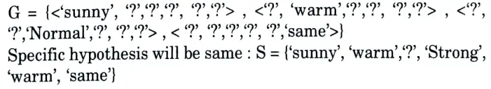
Step 5:
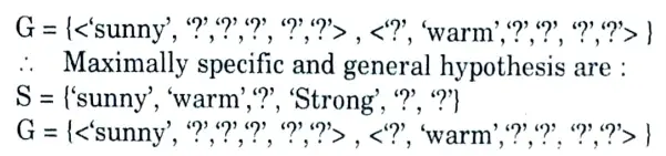
Instance 4 is positive so repeat step 3:

Discard the general hypothesis set which is contradicting with a resultant specific hypothesis. Here humidity and forecast attribute is contradicting.
Section 4: Algorithmic convergence & Generalization property of ANN
a. Comment on the Algorithmic convergence & Generalization property of ANN.
Ans. Algorithmic convergence of ANN:
- 1. In general, convergence refers to a process’s values that tend to change with time in terms of behaviour.
- 2. It is a practical notion when using optimisation methods.
- 3. By definition, an optimisation problem is one in which the goal is to identify a collection of inputs that would provide either the largest or smallest value possible for an objective function.
- 4. Optimization is an iterative process that generates a succession of potential solutions before concluding with a final solution.
- 5. Convergence describes the behaviour or dynamics of an optimisation method that has reached a stable-point ultimate solution.
- 6. For algorithms that fit (learn) on a training dataset via an iterative optimisation process, such as artificial neural networks, the convergence of optimisation algorithms is a key idea in machine learning.
Generalization property of ANN:
- 1. The generalization ability of Artificial Neural Networks (ANN) is largely responsible for their performance.
- 2. The ANN’s capacity to handle unknown data is a generalization.
- 3. System complexity and network training largely impact the network’s ability to generalize.
- 4. When the network has been overtrained or the system complexity (or degree of freedom) is disproportionately greater than the training data, poor generalization is shown.
- 5. A smaller network which can fit the data will have the k good generalization ability.
- 6. One of the promising techniques for lowering a network’s degree of freedom and enhancing its generalization is network parameter pruning.
b. Discuss the following issues in Decision Tree Learning:
1. Overfitting the data
2. Guarding against bad attribute choices
3. Handling continuous valued attributes
4. Handling missing attribute values
5. Handling attributes with differing costs
Ans. A. Overfitting the data:
- 1. When we train a machine learning algorithm with a lot of data, we say that it is overfitted.
- 2. As a model is trained with a large amount of data, it begins to learn from the errors and noise in our data set.
- 3. Next, due to excessive noise and detail, the model fails to appropriately classify the input.
- 4. Non-parametric and non-linear approaches are the sources of overfitting.
- 5. If we have linear data, employing a linear algorithm is one way to prevent overfitting, as is using decision tree characteristics like the maximal depth.
B. Guarding against bad attribute choices:
- 1. The main problem in implementing a decision tree is figuring out which properties we should take into account as the root node at each level.
- 2. Handling this is known as attribute selection.
- 3. As an example consider the attribute Date, which has a very large number of possible values.
- 4. What is wrong with the attribute Date ? Simply put, it has so many possible values that it is bound to separate the training examples into very small subsets.
- 5. Because of this, it will have a very high information gain relative to the training examples.
- 6. To guard against bad attribute choice we use gain ratio.
- 7. By using a term termed split information that is sensitive to how broadly and evenly the attribute splits the data, the gain ratio metric penalizes attributes like Date.
C. Handling continuous valued attributes:
- 1. In the ID3 algorithm, the attributes put to the test in the tree’s decision nodes must have discrete values.
- 2. It is simple to eliminate the aforementioned constraint in order to include continuous valued choice attributes in the learning tree.
- 3. For an attribute A that is continuous-valued, the algorithm can dynamically create a new boolean attribute A, that is true if A < c and false otherwise.
- 4. The only catch is how to select the best value for the threshold c.
D. Handling missing attribute values:
- 1. In some circumstances, the data that is currently accessible may lack values for some attributes.
- 2. In these situations, it is typical to estimate the value of the missing attribute using examples where the value of the characteristic is known.
- 3. Assigning the value that appears the most frequently in training samples at node n is one method for handling a missing attribute value.
- 4. A second, more complex procedure is to assign a probability to each of the possible values of A.
E. Handling attributes with differing costs:
- 1. The instance properties in some learning tasks could come at a price.
- 2. The prices of these characteristics range widely.
- 3. For these types of assignments, we would like decision trees that use low-cost attributes wherever possible, relying on high-cost attributes only when absolutely necessary to provide accurate classifications.
- 4. By including a cost term in the attribute selection measure, the ID3 algorithm can be changed to take attribute costs into account.
Section 5: Naive Bayesian Classifier
a. How is Naive Bayesian Classifier different from Bayesian Classifier ?
Ans. 1. In certain educational objectives, the instance properties may have 1. Naive Bayes and Bayes theorem vary in that the former implies conditional independence while the latter does not.
2. The Naive Bayes classifier is an approximate form of the Bayes classifier in which the features are assumed to be conditionally independent given the class rather than having their entire conditional distribution modeled.
3. A Bayes classifier is best interpreted as a decision rule.
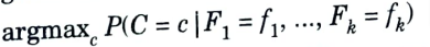
4. Suppose we seek to estimate the class of an observation given a vector of features. Denote the class C and the vector of features (F1, F2,…..,Fk).5. Given a probability model underlying the data (that is, given the joint distribution of (C, F1, F2,…..,Fk), the Bayes classification function chooses a class by maximizing the probability of the class given the observed features:
6. Although the Bayes classifier seems appealing, in practice the quantity
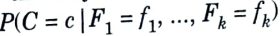
is very difficult to compute.
7. We can make it a bit easier by applying Bayes theorem and ignoring the resulting denominator, which is a constant.
8. Then we have the slightly better
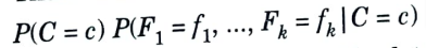
but this is often still intractable: lots of observations are required to estimate these conditional distributions, and this gets worse as k increases.
9. As a consequence, an approximation is used : we pretend
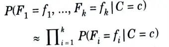
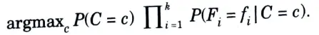
10. This is a pretty naive approximation, but in practice it works surprisingly well. Substituting this into the Bayes classifier yields the naive Bayes classifier:
b. Explain the role of Central Limit Theorem Approach for deriving Confidence Interval.
Ans.
- 1. It is possible to calculate an interval within which the population mean should fall. This tells us how accurate we are.
- 2. But, as we can never be completely certain of anything, we must assign a level of confidence to this interval.
- 3. We begin by taking into account a population’s mean confidence interval.
- 4. You may estimate how much variance will show up in repeated observations and statistical calculations using confidence intervals.
- 5. They estimate how much trust you may put in any of your measurements or statistical inferences from samples using the central limit theorem.
- 6. The central limit theorem states that the sampling distribution of the mean approaches a normal distribution, as the sample size increases.
- 7. This fact holds especially true for sample sizes over 30.
- 8. Therefore, as a sample size increases, the sample mean and standard deviation will be closer in value to the population mean 𝜇 and standard deviation 𝜎.
Section 6: Probably Approximately Correct (PAC)
a. Write short notes on Probably Approximately Correct (PAC) learning model.
Ans.
- 1. A paradigm for mathematically analyzing machine learning is known as probably approximately correct (PAC) learning.
- 2. Harvard University professor Leslie Valiant made the suggestion in 1984.
- 3. The PAC model belongs to the category of learning models that emphasizes example-based learning.
- 4. In this framework, the student is given samples and is required to choose one generalization function (referred to as the hypothesis) from a set of potential functions.
- 5. With a high degree of probability, the chosen function should have little generalization error.
- 6. The learner must be able to understand the topic regardless of the sample distribution, success probability, or approximation ratio used.
- 7. The model was later extended to treat noise (misclassified samples).
- 8. The PAC framework’s application of notions from computational complexity theory to machine learning is a significant advance.
- 9. In particular, the learner is required to implement an efficient approach and locate efficient functions.
b. Discuss various Mistake Bound Model of Learning.
Ans. Following are the various Mistake Bound Model of Learning:
A. Mistake Bound Model: Find-S
1. Instances drawn at random from X according to distribution D.
2. Learner must classify each instance before receiving correct classification from teacher.
3. Consider Find-S when H = conjunction of boolean literals.
i. Initialize h to the most specific hypothesis
ii. For each positive training instance x, remove from h any literal that is not satisfied by x.
iii. Output hypothesis h.
4. How many mistakes before converging to correct h ? n +1.
5. The first hypothesis eliminates n terms, each subsequent mistake will eliminate at least one more term.
B. Mistake Bound Model: Halving Algorithm
1. Consider the Halving Algorithm
i. Learn concept using version space Candidate-Elimination algorithm.
ii. Classify new instances by majority vote of version space members.
2. How many mistakes before converging to correct h ? log 2 |H|.
3. Every mistake eliminates at least half of the hypothesis from the version space (majority vote).
4. The version space starts at |H|.
C. Optimal Mistake Bounds:
1. Let Cbe an arbitrary nonempty concept class.
2. The optimal mistake bound for C, denoted Opt(C), is the minimum over all possible learning algorithms A of MA(C).
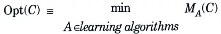
3. This definition states that Opt(C) is the number of mistakes made for the hardest target concept in C, using the hardest training sequence, by the best algorithm.
4. Now, for any concept class C, there is an interesting relationship among the optimal mist ake bound for C, the bound of the HALVING algorithm, and the VC dimension of C, namely

Section 7: Learn-one Rule Algorithm
a. What is the significance of Learn-one Rule Algorithm ?
Ans. 1. The sequential learning algorithm uses this technique to teach rules.
2. It provides one rule that addresses at least some examples.
3. But, what makes it really effective is its capacity to establish relationships between the provided qualities, thereby including a wider hypothesis space.
4. The Learn-One-Rule method uses a greedy searching paradigm to find the rules, which results in a very low coverage but great accuracy.
5. It organizes all the encouraging examples for a specific situation.
6. It involves a PERFORMANCE method that calculates the performance of each candidate hypothesis, (i.e., how well the hypothesis matches the given set of examples in the training data.
Performance(NewRule, h):
h-examples = the set of rules that match h
return (h-examples)
7. It starts with the most general rule precondition, then greedily adds the variable that most improves performance measured over the training examples.
b. Describe a prototypical genetic algorithm along with various operations possible in it.
Ans. Table :
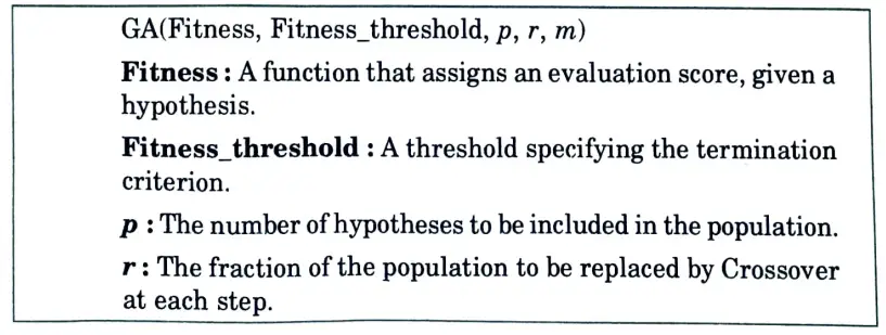
- 1. A prototypical genetic algorithm is described in Table.
- 2. The parameters that determine how successor populations are to be generated are the fitness function for ranking candidate hypotheses, a threshold defining an acceptable level of fitness for terminating the algorithm, the size of the population to be maintained, and the fraction of the population that will be replaced at each generation and the mutation rate.
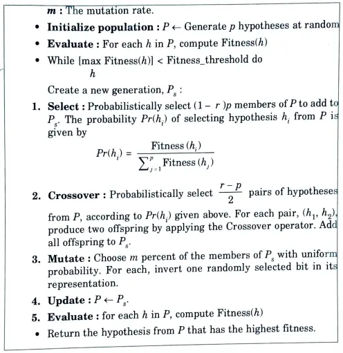
- 3. This algorithm generates a new generation of hypotheses based on the current population with each iteration of the main loop.
- 4. To start, a predetermined number of present population hypothese are chosen to be a part of the upcoming generation.
- 5. These are selected probabilistically, where the probability of selecting hypothesis hi is given by
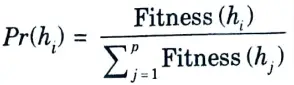
- 6. As a result, the likelihood that a hypothesis will be chosen is inversely proportional to the fitness of the competing hypotheses in the present population and is proportional to the fitness of the hypothesis being considered.
- 7. Following the selection of these members of the current generation for inclusion in the population of the following generation, more individuals are produced via a crossover operation.
- 8. When this crossover procedure has produced new members, the next generation population now has the desired number of individuals.
- 9. At this stage, a predetermined percentage of these members, m, are randomly selected, and random mutations are all carried out to change these members.
- 10. As a result, this GA method runs a parallel, randomized beam search to find hypotheses that perform well based on the fitness function.
6 thoughts on “Machine Learning Techniques: Aktu Question Paper with Quantum Notes”