
Information Theory and Coding: B.Tech AKTU question paper with answers presents a comprehensive set of exam-style questions and detailed solutions, aiding students in preparing for information theory and coding examinations
Dudes 🤔.. You want more useful details regarding this subject. Please keep in mind this as well.

Important Questions For Information Theory and Coding:
*Quantum          *B.tech-Syllabus
*Circulars           *B.tech AKTU RESULT
* Btech 4th Year
Section A: Short Question Information Theory and Coding
a. Describe the concept information rate and redundancy as referred to information transmission.
Ans. Information rate :
Let us suppose that, the symbols are emitted by the source at a fixed time rate “rs” symbols/sec. The average source information rate Rs in bits/sec is defeat as the product of the average information content per symbol and the message symbol rate “rs“.
∴ Rs =rs H(s) bits/sec or BPS
Redundancy :
In Information theory, redundancy measures the fractional difference between the entropy H(X) of an ensemble X, and its maximum possible value log { |log AX|}.
b. Write the expression for maximum entropy.
Ans.
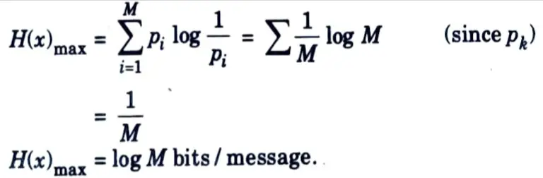
c. Evaluate the entropy for equal probable events.
Ans. For a finite set of states, the entropy reaches maximum when all the outcomes of an event are equally probable.
d. Define memory order of convolution code ?
Ans. A convolutional encoder continually processes the information sequence. The n-bit encoder output at any one time is determined not only by the k-bit information sequence, but also by the m prior input blocks, implying that a convolutional encoder has an m-bit memory order. An (n, k, m) convolutional code is the collection of sequences created by a k-input, n-output encoder of memory order m.
e. Calculate channel capacity of error free channel.
Ans.
- 1. Shannon’s renowned channel-capacity theorem combines the effects of bandwidth and signal-to-noise ratio and relates them to a variable ‘C’, which he calls the channel capacity and reflects the highest rate of information transmission supported by a channel.
- 2. For a channel of bandwidth B hertz with additive noise spectral density N0/2 (two-sided) he has shown that
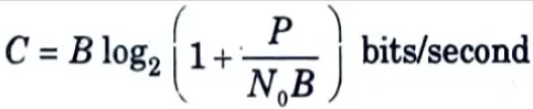
where, P is the average transmitted power.
- 3. He has shown that it is possible to have error-free transmission over such a noisy channel as long as the rate of transmission Rb, is less than the channel capacity C.
f. What are the various ways of representing convolutional codes ?
Ans. There are several methods for representing a convolutional code in graphical form :
- i. State transition diagram.
- ii. Tree diagram
- iii. Trellis diagram
g. State competitive optimality ?
Ans. Competitive optimality (CO) refers to a probabilistic strategy to estimating the likelihood of a source. Given the likelihood of a source, a uniquely decodable (UD) source code can be designed to minimise the predicted codelength.
h. What is expected length L(C) of a source code C(x)?
Ans. The expected length of a source code C(x) for a random variable X with probability mass function p(x) is given by
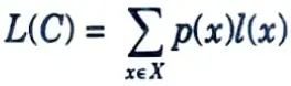
where l(x) is the length of the codeword associated with x.
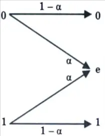
i. Draw diagram of binary erasure channel.
Ans. Binary erasure channel :
Section B : Repeated Questions of Information Theory and Coding
a. Calculate mutual information and capacity of binary symmetric channel.
Ans. Binary symmetric channel :
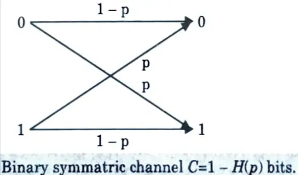
- 1. Consider the binary symmetric channel (BSC), which is shown in Fig.
- 2. This is a binary channel in which the input symbols are complemented with probability p.
- 3. When an error occurs, a 0 is received as a 1, and vice-versa. The bits received do not reveal where the errors have occurred.
- 4. We bound the mutual information by
I(X ; Y) = H(Y) – H(Y|X)
= H(Y) – ∑ p(x) H(Y | X = x)
= H(Y) – ∑ p(x) H(p)
= H(Y) – H(p) ≤ 1 – H(p)
where the last inequality follows because Y is a binary random variable.
- 5. Equality is achieved when the input distribution is uniform
- 6. Hence, the information capacity of a binary symmetric channel with parameter p is
C =1-H(p) bits.
b. State and prove AEP.
Ans. AEP Theorem :
If X1, X2,…., are i.i.d ~ p(x), then

Proof :
1. Functions of independent random variables are also independent random variables.
2. Thus, since the Xi are i.i.d, so are log p(Xi). Hence by the weak law of large numbers,

= – E log p(X) in probability …(2.1.3)
= H (X) …(2.1.4)
which proves the theorem.
c. Explain Jensen’s Inequality and its consequences.
Ans. Jensen’s inequality :
1. If f is a convex function and X is a random variable.
Ef (X) ≥ f(E X) ….(1.21.1)
2. Moreover, if f is strictly convex, the equality in eq. (1.21.1) implies that X = EX with probability 1 (i.e., X is a constant).
3. For a two-mass-point distribution, the inequality (1.21.1) becomes
p1f(x1) + p2f(x2) ≥ f(p1x1 + p2x2) ….(1.21.2)
which follows directly from the definition of convex functions.
4. Suppose that the theorem is true for distributions with k – 1 mass points. Then writing p’i = pi / (1 – pk) for i = 1, 2, …, k – 1, we have
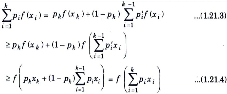
where the first inequality follows from the induction hypothesis and the second follows from the definition of convexity.
Consequences :
1. Information inequality : Let p(x), q(x), x ∈ X, be two probability mass functions. Then
D(p || q) ≥ 0 ….(1.21.5)
with equality if and only if p(x) = q(x) for all x.
2. H(X) ≤ log |χ|, where |χ| denotes the number of elements in the range of X, with equality if and only χ has a uniform distribution over χ.
3. H (X | Y) ≤ H(X)
with equality if and only if X and Y are independent.
4. Independence bound on entropy
X1, X2, …Xn be drawn according to p(x1, x2, ….xn). Then
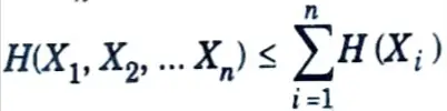
with equality if and only if the Xi are independent.
d. Describe hamming codes and determine hamming bound.
Ans. Hamming codes: Consider a family of (n, k) linear block codes that ave the following properties :
i. Block length n = 2m – 1.
ii. Number of message bits k = 2m – m -1.
iii. Number of parity bits m = n – k where m ≥ 3.
The block codes having above properties are known as Hamming codes.
e. Explain Golay codes ?
Ans.
- 1. The Golay code is a perfect linear error-correcting code.
- 2. There are two essentially distinct versions of the Golay code : a binary version and a ternary version.
- 3. The binary version G23 is a (23, 12, 7) binary linear code consisting of 212 = 4096 codewords of length 23 and minimum distance 7.
- 4. The terHary version is a (11, 6, 5) ternary linear code, consisting of 36 = 729 codewords of length 11 with minimum distance 5.
- 5. A parity check matrix for the binary Golay code is given by the matrix H = (MI11), where I11 is the 11 x 11 identity matrix and M is the 11 x 12 matrix.
- 6. This code is able to correct up to 3 corrupted bits per block of 12 and detect more. 7. By adding a parity check bit to each codeword in G23, the extended Golay code G24, which is a nearly perfect [24,12,8] binary linear code, is obtained.
Section 3 : Fano’s Inequality in Information Theory and Coding
a. State and prove Fano’s inequality.
Ans. 1. Fano’s inequality relates the probability of error in guessing the random variable X to its conditional entropy H(X|Y).
2. It will be crucial in proving the converse to Shannon’s channel capacity theorem. We know that the conditional entropy of a random variable X given another variable Y is zero if and only if X is a function of Y.
3. Hence, we can estimate X from Y with zero probability of error if and only if H(X|Y) = 0.
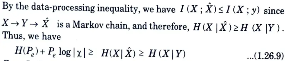
Fano’s inequality :
1. For any estimator X̂ such that
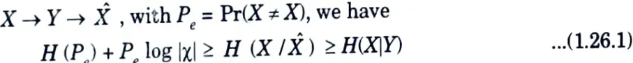
2. This inequality can be weakened to
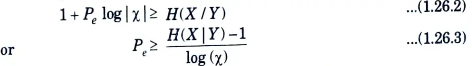
Note that Pe = 0 implies that H(X|Y) = 0, as intuition suggests.
3. We first ignore the role of Y and prove the first inequality in eg (1.26.1) error random variable.
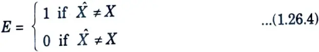
4. Then, using the chain rule for entropies to expand H (E ,X | X̂) in two different ways, we have
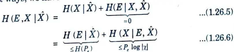
Since, conditioning reduces entropy, H (E | X̂) ≤ H(E) = H(Pe).
5. Now, since E is a function of X and X̂, the conditional entropy H (E | X, X̂) is equal to 0. Also, since E is a binary-valued random variable, H(E) = H(Pe).
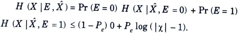
6. The remaining term, H (X | E,X̂), can be bounded as follows :
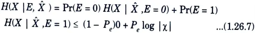
7. Since given E = 0, X = X̂ and given E = 1, we can upper bound the conditional entropy by the log of the number of possible outcomes. Combining these results, we obtain

Case I: For any two random variables X and Y, let p = Pr(X ≠ Y )

Proof : Let X̂ = Y in Fano’s inequality.
For any two random variables X and Y, if the estimator g(Y) takes values in the set 𝛘, we can strengthen the inequality slightly by replacing log |𝛘| with log (|𝛘| – 1).
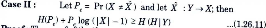
Proof: The proof of the theorem goes through without change, except that
since, given F = 0, X = Ĥ and given E = 1, the range of possible X
outcomes is |X| – 1, we can upper bound the conditional entropy by the log (|X| – 1), the logarithm of the number of possible outcomes. Substituting this provides us with the stronger inequality.
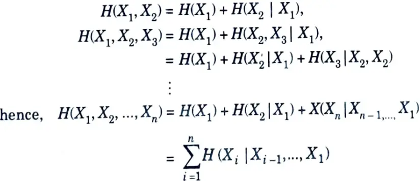
b. State and prove chain rule of entropy and relative entropy.
Ans. Chain rule of entropy :
Let X1, X2,….Xn be drawn according to p(x1, x2,….xn). Then,
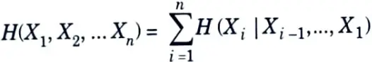
Proof: By repeated application of the two-variable expansion rule for entropies, we have
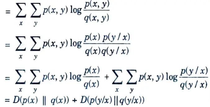
Chain rule of relative entropy :
D(p(x, y) || q(x, y)) = D (p(x) || q(x)) + D (p(y|x) || q(y|x))
Proof : Dp(x, y) || q(x, y))
Section 4 : Optimal Code Length in Information Theory and Coding
a. Determine the bound on optimal code length.
Ans. 1. We now demonstrate a code that achieves an expected description length L within 1 bit of the lower bound; that is,
H (X) ≤ L < H (X) + 1 …(.2.12.1)
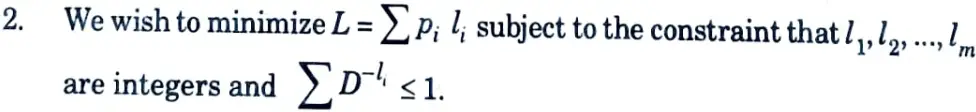
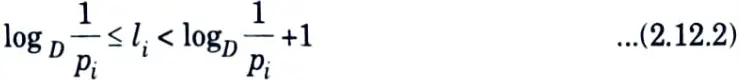
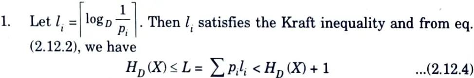
3. The choice of word lengths
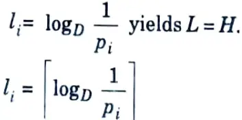
where

is the smallest integer ≥ x.
4. These lengths satisfy the Kraft inequality since
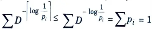
5. This choice of codeword lengths satisfies
Multiplying by pi and summing over i, we obtain
HD (X) ≤ L< HD (X) + 1 ….(2.12.3)
Since, an optimal code can only be better than this code, we have the following theorem.
Theorem: Let l*1, l*2,….l*m be optimal codeword lengths for a source distribution p and a D-ary alphabet, and let L be the associated expected length of an optimal code
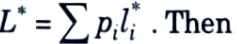
HD (X) ≤ L*< HD (X) + 1 ….(2.12.3)
Proof :
But since L*, the expected length of the optimal code, is less than

2. Define Ln to be the expected codeword length per input symbol, that is, if l (x1, x2,…..xn) is the length of the binary codeword associated with (x1, x2,….xn), we assume that D = 2, for simplicity, then
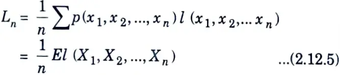
3. We can now apply the bounds derived above to the code :
Dividing eq. (2.12.6) by n, we obtain
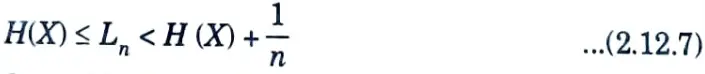
Hence, by using large block length we can achieve an expected code length per symbol arbitrarily close to the entropy.
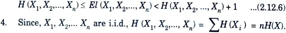
5. We can use the same argument for a sequence of symbols from a stochastic process that is not necessarily i.i.d.
6. In this case, we still have the bound
H(X1, X2,…..Xn) ≤ El (X1, X2,…..Xn) < H(X1, X2,…..Xn) + 1
Dividing by n again and defining Ln to be the expected description length per symbol, we obtain
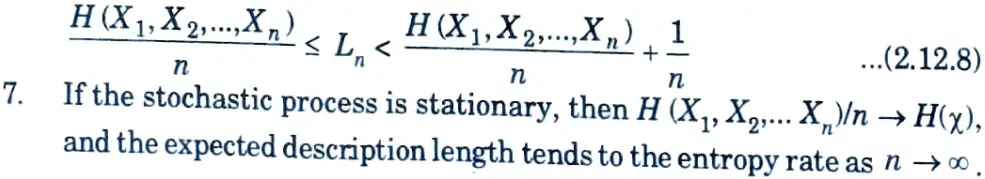
Thus, we have the following theorem :
Theorem :
The minimum expected codeword length per symbol satisfies,
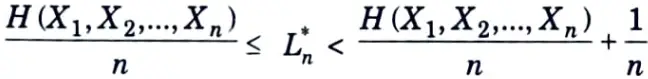
Moreover, if X1, X2, ….Xn is a stationary stochastic process,
L*n → H(X)where H(𝛘) is the entropy rate of the process.
b. Explain Shannon Fano Elias coding.
Ans. 1. Codeword length
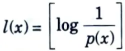
can be used to construct a uniquely decodable code for the source.
2. The cumulative distribution function F(x) is defined as,
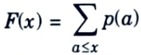
It can also be defined as modified cumulative distribution function as,
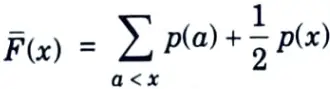
where F(bar)(x) denotes the sum of the probabilities of all symbols less than x plus half the probability of the symbol x. Since the random variable is discrete, the cumulative distribution function consists of steps of size p(x).
3. F(bar)(x) is a real num ber expressible only by an infinite number of bits.
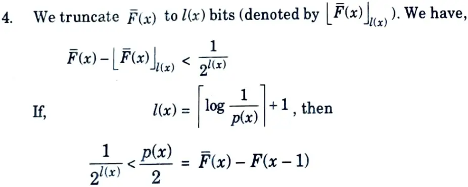
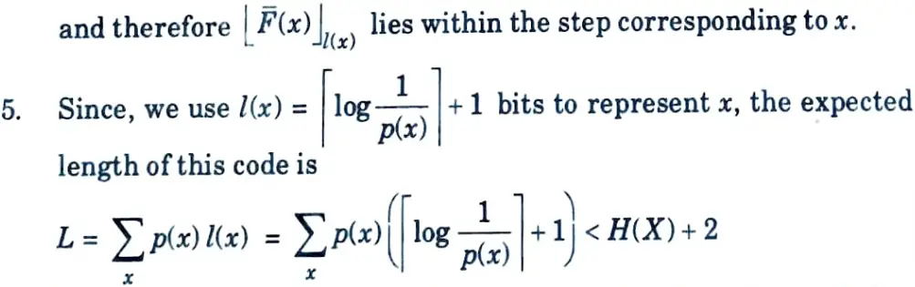
Thus, this coding scheme achieves an average codeword length that is within 2 bits of the entropy.
Section 5 : Jointly Typical Sequences in Information Theory and Coding
a. Explait channel coding theorem.
Ans. For a discrete memory-less channel, all rates below capacity C are achievable. Specifically, for every rate R < C, there exists a sequence of (2nR, n) codes with maximum probability of error 𝛌(n) → 0.
Conversely, any sequence of (2nR, n) codes with 𝛌(n) → 0 must have R ≤ C.
It is also called Shannon’s second theorem.
b. Briefly explain the properties of jointly typical sequences.
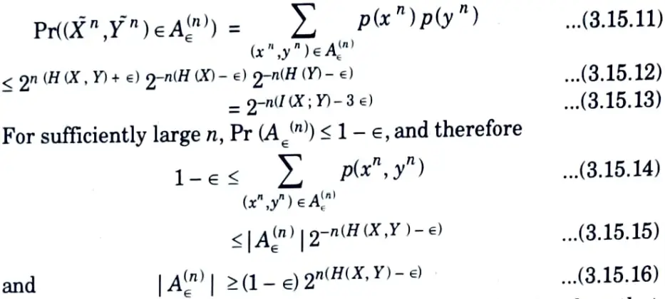
Ans. Theorem :Let (xn, yn) be sequences of length n drawn independent identical distribution (i.i.d) according to
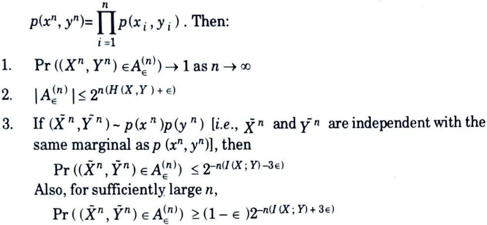
Proof :
1. By the weak law of large numbers,
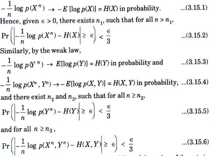
Choosing n > max {n1, n2, n3), the probability of the union of the sets in eg. (3.15.2), (3.15.5), and (3.15.6) must be less than ∈. Hence, for n sufficiently large, the probability of the set A∈(n) is greater than 1 – ∈, establishing the first part of the theorem.
2. To prove the second part of the theorem, we have
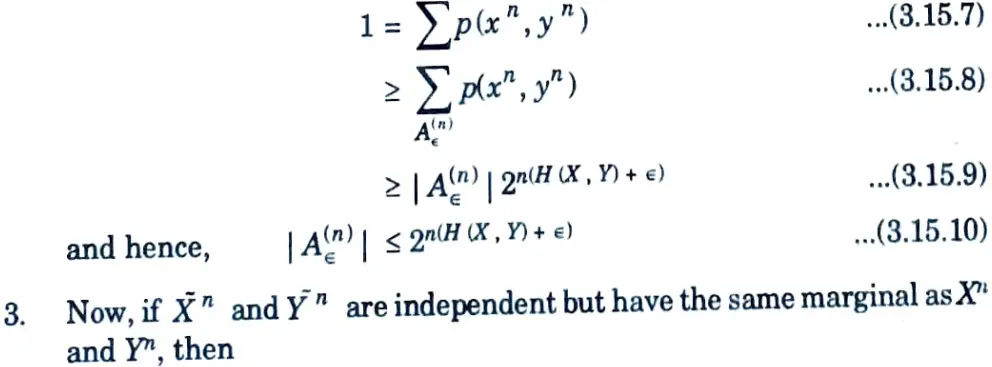
By similar arguments to the upper bound above, we can also show that for n sufficiently large,
4. The jointly typical set is illustrated in Fig. 3.15.1
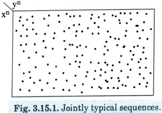
5. They are about 2n H(X) typical X sequence and about 2n H(Y) typical Y sequences. However, since there are only 2n H(X, Y)jointly typical sequences, not all pairs of typical Xn and typical Yn are also jointly typical.
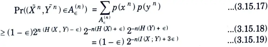
6. The probability that randomly chosen pair is jointly typical is about 2-n I(X;Y).
Section 6 : Soft-Decision Decoding in Information Theory and Coding
a. Explain soft-decision decoding with example.
Ans.
- 1. The output of the demodulator is always a 0 or a 1. Such a demodulator is said to make hard decisions. A demodulator that is not constrained to return 0 or 1 but is allowed to return a third symbol, say X, is said to make soft decisions.
- 2. A soft decision is made whenever the demodulator input is so noisy that a 0 and 1 are equiprobable. The symbol X is referred to as an erasure and Fig. 4.16.1, shows a channel that includes erasures.
- 3. An erasure is defined as an error whose position is known but whose size is unknown, and which is assumed to be 1/2 the distance between 0 and 1. (i.e., equidistant from 0 and 1).
- 4. A hard-decision demodulator provides no indication of the quality of the Os and ls entering the decoder.
- 5. Based on the error-control code, the decoder determines the presence or absence of errors.
- 6. A soft-decision demodulator, on the other hand, supplies additional information to the decoder that can be used to improve error control. If the decoder detects an error, any erasures in the word being decoded are the bits that are most likely to be incorrect.
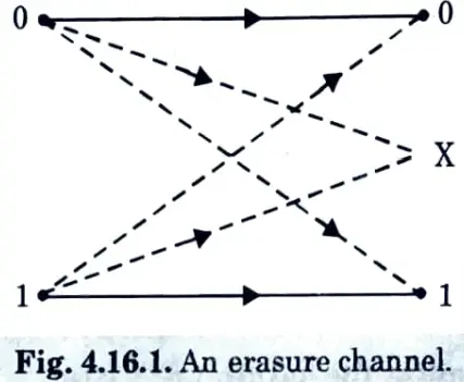
Table : Error and erasure correction for dmin 10.
| t’ | s’ |
| 0 | 9 |
| 1 | 7 |
| 2 | 5 |
| 3 | 3 |
| 4 | 1 |
- 7. Consider the (8, 7) even parity code and let’s assume that the input to the decoder is v = (10 010100). The parity of v is odd and therefore the decoder knows that at least l error has occurred.
- 8. Based on the parity of v alone the decoder has no way of establishing the position of the error, or errors inu. Consider now a decoder whose input is taken from a soft-decision demodulator and let v = (0 1 1 1 0 X 1 1) be the decoder input.
- 9. The parity of v is incorrect but here it is reasonable to assume that the position of the erasure gives the bit that is most likely to be in error.
- 10. If the erasure is assumed to have a 0 value then v still has the wrong parity. However setting X = 1 gives v = (0 1 1 1 0 1 1 1) which has the correct parity and can be taken as the most likely even-parity codeword that v corresponds to.
- 11. If v has the correct parity and contains an erasure, then the erasure is set to 0 or 1 as so to preserve the correct parity, for example given v = (1 X 0 0 0 1 0 0) we would set X = 0. If v contains single erasure, and no other errors, then single-error correction is guaranteed.
- 12. The (8, 7) even-parity code is an error-detecting code, it has no error correcting capability.
- 13. The combination of error-control coding with soft-decision demodulation is referred to as soft-decision decoding.
- 14. It can be shown that for a code with minimum distance dmin any pattern of t’ errors and s’ erasures can be corrected providing
- 2t’ + s’ ≤ dmin – 1
- 15. Table, shows values of t’ and s’ for dmin = 10. The (8, 7) even-parity code has dmin = 2 and t = 0 therefore only 1 erasure can be corrected.
- 16. The (7, 4) code, with dmin = 3, cannot correct erasures when used for error correction, but can correct upto 2 erasures if error correction is not carried out.
- 17. There are benefits to be gained by using soft-decision demodulators that are not constrained to return 0 or l but can return erasures. Further benefits can be gained using demodulators that can assign a bit quality to each bit.
- 18. Here, the demodulator decides whether each bit is a 0 or l and assign a bit quality that indicates how good each bit is. A bit that is clear cut 0 or 1 would be assigned a high bit quality, while a bit that is only just a 0 or 1 is given a low bit quality. In the case where a bit is equally likely to be a 0 or a 1 then an erasure is returned.
- 19. The decoder then makes its decision not just on the basis of the bit values, 0, 1 or X but also on the quality associated with each bit. The use of bit-quality information can give considerable coding gains, but is at the expense of increased complexity for both the demodulator and the decoder.
Section 7 : Aktu Solved Important Questions in Information Theory and Coding
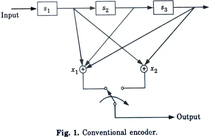
a. Using 3 stage shift register and 2 stage Modulo-2 adder with impulse response of paths (111) and (101), draw trellis diagram and if the transmitted code is 00000000 and received code have error on 2nd and 6th bit due to channel noise, then detect and correct the errors by using Viterbi decoding of the convolution code.
Ans.
A. To determine dimension of the code :
1. For every message bit (k = 1), two output bits (n = 2) are generated.

2. Since there are three stages in the shift register, every message bit will affect output for three successive shifts. Hence constraint length, K = 3. Thus, k = 1, n = 2 and K = 3
3. In the above figure observe that,
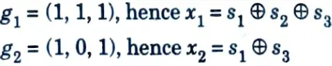
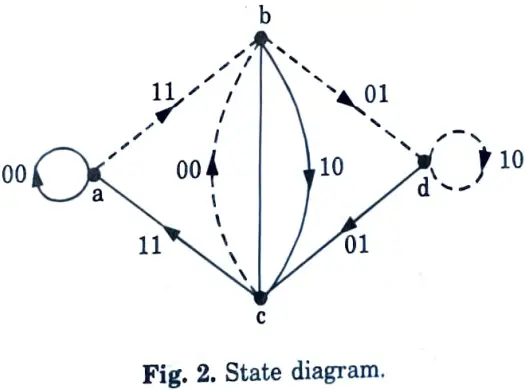
B. To obtain the state diagram :
1. First, let us define the states of the encoder.
s3 s2 = 00, state ‘a’
s3 s2 = 01, state ‘b’
s3 s2 = 10, state ‘c’
s3 s2 = 11, state ‘d’
2. A table is prepared that lists state transitions, message input and 00 outputs. The table is as follows:
Table 1. State transition table
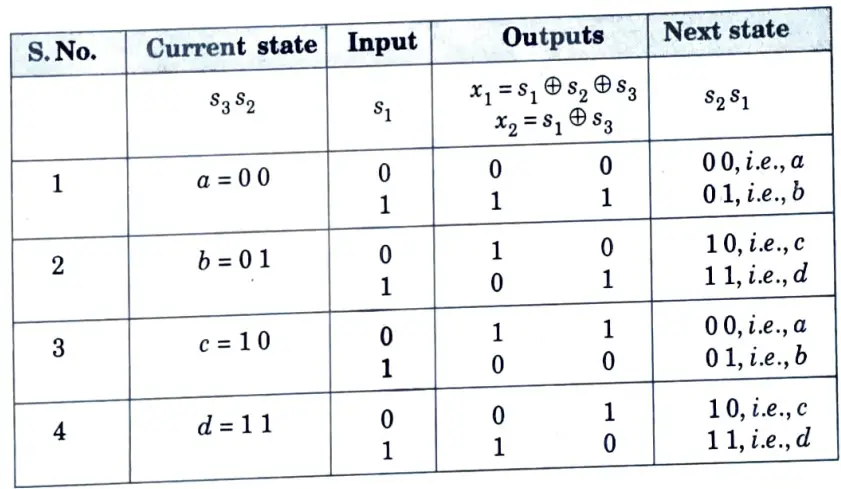
3. Based on above table, the state diagram can be prepared easily. It is shown in Fig. 2.
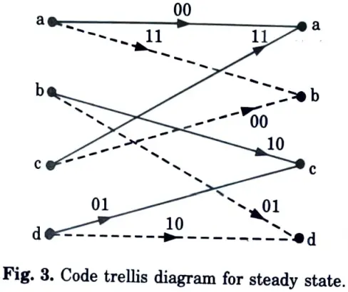
C. To obtain trellis diagram for steady state :
1. From Table 1, the code trellis diagram can be prepared. It is steady state diagram. It is shown in Fig. 3.
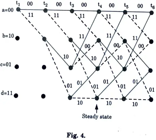
D. Termination of trellis to all zero state :
1. Fig. 4 shows the trellis diagram for first four received set of symbols. It begins with state a = 00.
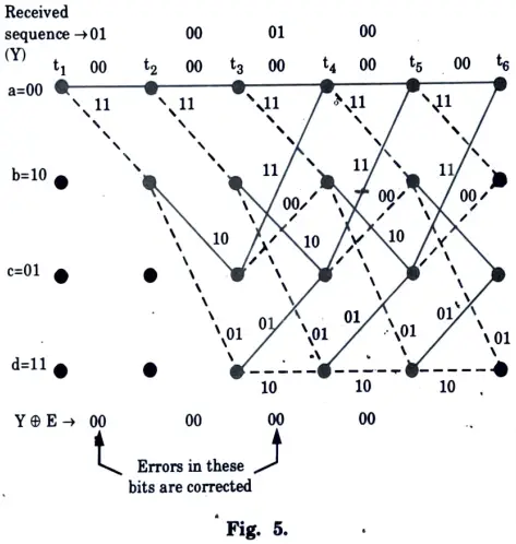
E. Detection and correction of error by using Viterbi algorithm :
1. Based upon code trellis of Fig. 3, the trellis diagram is shown in Fig. 5 for multiple stages.
2. The diagram begins from node t1.
3. The outputs and metric are marked along each branch. The cumulative metric are also marked near every node.
4. In Fig. 5 observe that the path, t1 – t2 – t3 – t4 – t5 – t6 is maximum likelyhood path. This path has lowest metric, compared to all other paths. Hence it is maximum likelyhood path.
5. Output due to this path is 00 00 00 00 … This shows that two errors at 2nd and 6th bit positions are corrected by Viterbi algorithm.
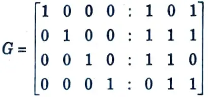
b. For the given generator polynomial g(x) = 1+ x + x3 find the generator matrix G for a symmetric (7, 4) cyclic code and find the systematic cyclic code for message bits 1010.
Ans. For this code n = 7, k = 4 and q = 3.
To determine generator matrix (G) :
The tth row of the generator matrix is given as,
pn-t + Rt(p) = QtG(p) and t = 1, 2, ….. k
We have obtained the generator matrix based on the above equation in example for the same generating polynomial. It is given by equation as,
Systematic cyclic code for message bits 1010 :
The message polynomial is m (x) = 1 + x2, and as n – k = 7 – 4 = 3, the polynomial x3m(x) = x3 + x5 is calculated. The polynomial division is done as follows :
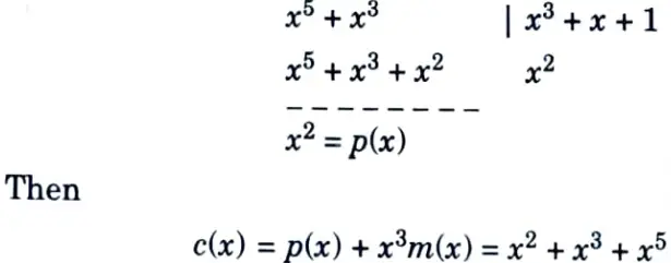
and so
c = (0011010)
1 thought on “Information Theory and Coding: Btech AKTU Question Paper Questions with Answer”