
Table Of Contents
In the B.Tech AKTU Quantum Book, learn about the practical Application of Soft Computing. Discover crucial applications, frequently asked questions, and essential notes for mastering this cutting-edge technology. Unit-2 Neural Network-II (Back Propagation Network)
Dudes 🤔.. You want more useful details regarding this subject. Please keep in mind this as well.

Important Questions For Application of Soft Computing:
*Quantum                *B.tech-Syllabus
*Circulars                 *B.tech AKTU RESULT
* Btech 3rd Year     * Aktu Solved Question Paper
Q1. What is the multilayer perceptron model? Explain it.
Ans.
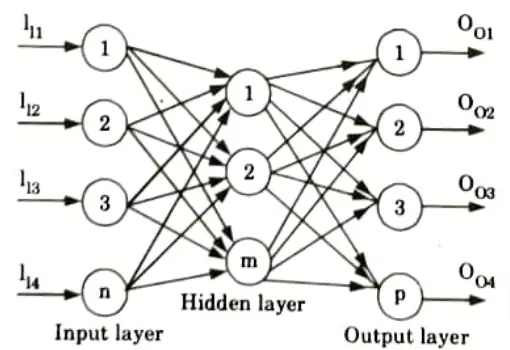
- 1. A multilayer perceptron is a feed forward artificial neural network class.
- 2. A multilayer perceptron model includes three layers: an input layer, an output layer, and a layer in between that is not directly connected to either the input or the output and is hence referred to as the hidden layer.
- 3. We utilise sigmoidal or squashed-S function for perceptrons in the input layer and linear transfer function for perceptrons in the hidden and output layers.
- 4. Because the input layer’s purpose is to distribute the values it receives to the next layer, it does not conduct a weighted sum or threshold.
- 5. The input-output mapping of multilayer perceptron is shown in Fig. and is represented by
- 6. Multilayer perceptron does not increase computational power over a single layer neural network unless there is a non-linear activation function between layers.
Q2. Differentiate single layer perceptron method and multilayer perceptron method.
Ans.
| S. No. | Single layer perceptron model | Multilayer perceptron model |
| 1. | It does not contain any hidden layer. | It contains one or more hidden layer. |
| 2. | It can learn only linear function. | It can learn linear and non-linear function. |
| 3. | It requires less training input. | It requires more number of training inputs. |
| 4. | Learning is faster. | Learning is slower. |
| 5. | Faster execution of the final network. | Slower execution of the final network. |
Q3. What are the back propagation learning methods ?
Ans. Learning methods of back propagation
- 1. Static back propagation :
- a. It is a back propagation network that generates a mapping of a static input to a static output.
- b. It can be used to address static classification problems such as optical character recognition.
- c. In static back propagation, the mapping is fast.
- 2. Recurrent back propagation:
- a. Recurrent back propagation is continued until a fixed value is reached.
- b. The mistake is then computed and propagated backward.
- c. In recurrent back propagation, it is non-static.
Q4. Write down the advantages and disadvantages of back propagation networks.
Ans. Advantage of back propagation networks/algorithm:
- 1. It is quick, straightforward, and simple to programme.
- 2. There are no tuning parameters (except for the number of input).
- 3. There is a batch weight update that gives a smoothing impact on the weight of correction terms.
- 4. The computing time is lowered if the weight specified at the start is minimal.
Disadvantage/Drawbacks of back propagation network/algorithm:
- 1. The actual performance of back propagation on a specific problem depends explicitly on the input data.
- 2. Back propagation is susceptible to noise and outliers.
- 3. Instead of a mini-batch, a fully matrix-based technique is employed for back propagation.
- 4. Once a network has learned one set of weights, every additional learning results in catastrophic forgetting.
Q5. Discuss the selection of various parameters in BPN.
Ans. Selection of various parameters in BPN (Back Propagation Network):
1. Number of hidden nodes:
- i. The leading criterion is to select the fewest nodes possible without impairing network performance, so that the memory required to store the weights is kept to a minimum.
- ii. When the number of concealed nodes equals the number of training patterns, learning may be accelerated.
- In such instances, the Back Propagation Network (BPN) recalls training patterns but loses all generalisation skills.
- iv. Hence, as far as generalization is concerned, the number of hidden nodes should be small compared to the number of training patterns (say 10:1).
2. Momentum coefficient (α):
- i The another method of reducing the training time is the use of momentum factor because it enhances the training process.
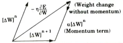
- ii. The momentum also overcomes the effect of local minima.
- iii. It will carry a weight change process through one or local minima and get it into global minima.
3. Sigmoidal gain (𝝺):
- i. When the weights become large and force the neuron to operate in a region where sigmoidal function is very flat, a better method of coping with network paralysis is to adjust the sigmoidal gain.
- ii. By decreasing this scaling factor, we effectively spread out sigmoidal function on wide range so that training proceeds faster.
4. Local minima:
- i. One of the most practical solutions is to introduce a shock that causes all weights to vary by specific or random amounts.
- ii. If this fails, the remedy is to re-randomize the weights and begin training again.
- iii. Simulated annealing is employed to keep training going until a local minima is reached.
- iv. Simulated annealing is then paused, and BPN proceeds until a global minimum is reached.
- v. In most cases, this two-stage procedure requires only a few simulated annealing cycles.
5. Learning coefficient (η):
- i. If the learning coefficient is negative, the change in weight vector position will deviate from the optimum weight vector position.
- ii. If the learning coefficient is zero, there is no learning; thus, the learning coefficient must be positive.
- iii. If the learning coefficient is more than one, the weight vector will overshoot and fluctuate from its optimal location.
- iv. As a result, the learning coefficient must be between 0 and 1.
Q6. Discuss how learning rate coefficient affects the back propagation training.
Ans.
- 1. The learning rate coefficient influences the rate of convergence by determining the amount of the weight adjustments made at each iteration.
- 2. A poor choice of coefficient can lead to a failure of convergence.
- 3. For the best outcomes, we should keep the coefficient constant across all iterations.
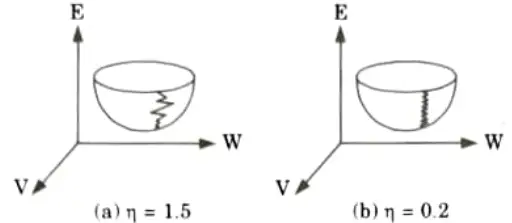
- 4. If the learning rate coefficient is too large, the search path will oscillate and converges more slowly than a direct descent as shown in Fig.(a).
- 5. If the coefficient is too small, the descent will progress in small steps significantly increasing the time to converge as shown in Fig.(b).

Application of Soft Computing Btech Quantum PDF, Syllabus, Important Questions
| Label | Link |
|---|---|
| Subject Syllabus | Syllabus |
| Short Questions | Short-question |
| Question paper – 2021-22 | 2021-22 |
Application of Soft Computing Quantum PDF | AKTU Quantum PDF:
| Quantum Series | Links |
| Quantum -2022-23 | 2022-23 |
AKTU Important Links | Btech Syllabus
| Link Name | Links |
|---|---|
| Btech AKTU Circulars | Links |
| Btech AKTU Syllabus | Links |
| Btech AKTU Student Dashboard | Student Dashboard |
| AKTU RESULT (One VIew) | Student Result |